
The Excel LOOKUP function performs an approximate match lookup in a one-column or one-row range, and returns the corresponding value from another one-column or one-row range. LOOKUP's default behavior makes it useful for solving certain problems in Excel.
=LOOKUP(lookup_value,lookup_vector,[result_vector])Use the LOOKUP function to look up a value in a one-column or one-row range, and retrieve a value from the same position in another one-column or one-row range. The lookup function has two forms, vector and array. The majority of this article describes the vector form, but the last example below illustrates the array form.
The LOOKUP function accepts three arguments: lookup_value, lookup_vector, and result_vector. The first argument, lookup_value, is the value to look for. The second argument, lookup_vector, is a one-row, or one-column range to search. LOOKUP assumes that lookup_vector is sorted in ascending order. The third argument, result_vector, is a one-row, or one-column range of results. Result_vector is optional. When result_vector is provided, LOOKUP locates a match in the lookup_vector, and returns the corresponding value from result_vector. If result_vector is not provided, LOOKUP returns the value of the match found in lookup_vector.
LOOKUP has default behaviors that make it useful when solving certain problems. For example, LOOKUP can be used to retrieve an approximate-matched value instead of a position and to find the last value in a row or column. LOOKUP assumes that values in lookup_vector are sorted in ascending order and always performs an approximate match. When LOOKUP can't find a match, it will match the next smallest value.
In the example shown above, the formula in cell F5 returns the value of the match found in column B. Note that result_vector is not provided:
=LOOKUP(F4,B5:B9) // returns match in level The formula in cell F6 returns the corresponding Tier value from column C. Notice in this case, both lookup_vector and result_vector are provided:
=LOOKUP(F4,B5:B9,C5:C9) // returns corresponding tier In both formulas, LOOKUP automatically performs an approximate match and it is therefore important that lookup_vector is sorted in ascending order.
LOOKUP can be used to get the value of the last filled (non-empty) cell in a column. In the screen below, the formula in F6 is:
=LOOKUP(2,1/(B:B<>""),B:B) 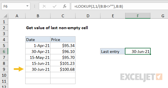
Note the use of a full column reference. This is not an intuitive formula, but it works well. The key to understanding this formula is to recognize that the lookup_value of 2 is deliberately larger than any values that will appear in the lookup_vector. Detailed explanation here.
Similar to the above example, the lookup function can be used to look up the latest price in data sorted in ascending order by date. In the screen below, the formula in G5 is:
=LOOKUP(2,1/(item=F5),price) where item (B5:B12) and price (D5:D12) are named ranges.
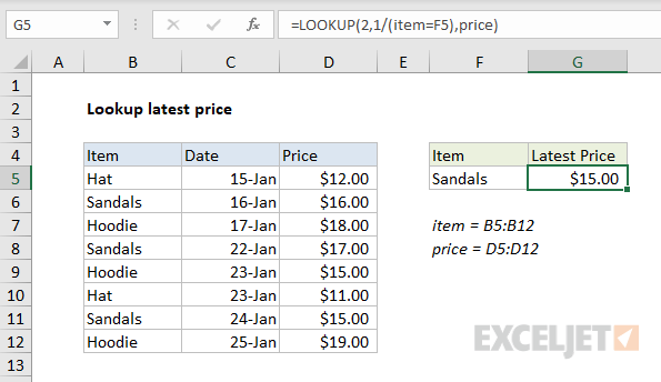
When lookup_value is greater than all values in lookup_array, default behavior is to "fall back" to the previous value. This formula exploits this behavior by creating an array that contains only 1s and errors, then deliberately looking for the value 2, which will never be found. More details here.
The LOOKUP function has an array form as well. In the array configuration, LOOKUP takes just two arguments: the lookup_value, and a single two-dimensional array:
LOOKUP(lookup_value, array) // array form In the array form, LOOKUP evaluates the array and automatically changes behavior based on the array dimensions. If the array is wider than tall, LOOKUP looks for the lookup value in the first row of the array (like HLOOKUP). If the array is taller than wide (or square), LOOKUP looks for the lookup value in the first column (like VLOOKUP). In either case, LOOKUP returns a value at the same position from the last row or column in the array. The example below shows how the array form works. The formula in F5 is configured to use a vertical array and the formula in F6 is configured to use a horizontal array:
=LOOKUP(E5,B5:C9) // vertical array =LOOKUP(E6,C11:G12) // horizontal array 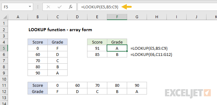
The vertical and horizontal arrays contain the same values; only the orientation is different.
Note: Microsoft discourages the use of the array form and suggests VLOOKUP and HLOOKUP as better options.

In the example shown, we have a set of order data that includes Date, Product, Name, and Amount. The data is sorted by date in ascending order. The goal is to look up the latest order for a given person by Name. In other words, we want the last match by name. The challenge is that Excel lookup.

The goal is to search through a cell for one of several specified values and return the last match found when one exists. The worksheet includes a list of colors in the range E5:E11 (which is named list ) and a series of short sentences in the range B5:B16. The task is to add a formula in column C.

The LOOKUP function does an approximate match lookup in one range, and returns the corresponding value in another. Although the table in this example includes both maximum and minimum values, we only need to use the minimum values. This is because when LOOKUP can't find a match, it will match the.

To do this, LOOKUP is configured as follows: Lookup values are ages in column C The lookup vector is the named range "age" (F5:F8) The result vector is the named range "group" (G5:G8) With this setup, LOOKUP performs an approximate match on the numeric values in column F, and returns the associated.

Note: the lookup_value of 2 is deliberately larger than any values in the lookup_vector, following the concept of bignum . Working from the inside out, the expression: (TEXT($B$5:$B$13,"mmyy")=TEXT(E5,"mmyy")) generates strings like "0117" using the values in column B and E, which are then compared.

Working from the inside out, the expression C5:G5<>"" returns an array of true and false values:

If you are new to the SUMIFS function, you can find a basic overview with many examples here . The SUMIFS function is designed to sum numeric values based on one or more criteria. In specific cases however, you may be able to use SUMIFS to "look up" a numeric value that meets required criteria. The.

In this example, the goal is to retrieve the last available close price for each symbol shown in column B. This can be done with the STOCKHISTORY function . The main purpose of STOCKHISTORY is to retrieve historical stock price information, and we need to make a few adjustments to prevent errors.
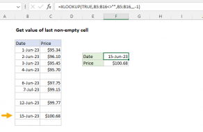
In this example, the goal is to get the last value in column B, even when data may contain empty cells. A secondary goal is to get the corresponding value in column C. This is useful for analyzing datasets where the most recent or last entry is significant. In the current version of Excel, a good.

The core of this formula is a basic lookup with INDEX: =INDEX(list,row) In other words, give INDEX the list and a row number, and INDEX will retrieve a value to add to the unique list. The hard work is figuring out the ROW number to give INDEX, so that we get unique values only. This is done with.

This formula uses the LOOKUP function to find and retrieve the last matching file name. The lookup value is 2, and the lookup_vector is created with this: 1/(ISNUMBER(FIND(G6,files))) Inside this snippet, the FIND function looks for the value in G6 inside the named range "files" (B5:B11). The.

This formula uses 4 named ranges, defined as follows: width=K6 height=K7 widths=B6:B11 heights=C5:H5 Conditional formatting is evaluated relative to every cell it is applied to, starting with the active cell in the selection, which is cell B5 in this case. To highlight the matching row, we use this.

In this example, the goal is to average the last 3 numeric values in a set of data. The best solution depends on the version of Excel you have available. In the current version of Excel, this can be nicely solved with a formula based on the AVERAGE function , the FILTER function , and the TAKE.

The LOOKUP function assumes data is sorted, and always does an approximate match. If the lookup value is greater than all values in the lookup array, default behavior is to "fall back" to the previous value. This formula exploits this behavior by creating an array that contains only 1s and errors.

In this video, we'll look at how to highlight approximate match lookups with conditional formatting. Here we have a simple lookup table that shows material costs for various heights and widths. The formula in K8 uses the INDEX and MATCH functions to retrieve the correct cost based on width and.
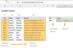
The Excel VLOOKUP function is used to retrieve information from a table using a lookup value. The lookup values must appear in the first column of the table, and the information to retrieve is specified by column number. VLOOKUP supports approximate and exact matching.

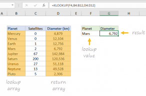
The Excel HLOOKUP function finds and retrieve a value from data in a horizontal table. The "H" in HLOOKUP stands for "horizontal", and lookup values must appear in the first row of the table, moving horizontally to the right. HLOOKUP supports approximate and exact matching, and.
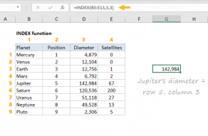
The Excel INDEX function returns the value at a given location in a range or array. You can use INDEX to retrieve individual values, or entire rows and columns. The MATCH function is often used together with INDEX to provide row and column numbers.
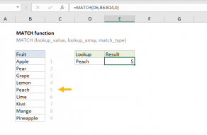
MATCH is an Excel function used to locate the position of a lookup value in a row, column, or table. MATCH supports approximate and exact matching, and wildcards (* ?) for partial matches. Often, MATCH is combined with the.
The Excel XLOOKUP function is a modern and flexible replacement for older functions like VLOOKUP, HLOOKUP, and LOOKUP. XLOOKUP supports approximate and exact matching, wildcards (* ?) for partial matches, and lookups in vertical or horizontal ranges.

The Excel XMATCH function performs a lookup and returns a position of a value in a range. It is a more robust and flexible successor to the MATCH function. XMATCH supports approximate and exact matching, reverse search, and wildcards (* ?) for partial matches. .
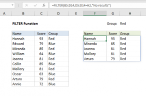
The Excel FILTER function is used to extract matching values from data based on one or more conditions. The output from FILTER is dynamic. If source data or criteria change, FILTER will return a new set of results. This makes FILTER a flexible way to isolate and inspect data without altering the.
Author
Hi - I'm Dave Bruns, and I run Exceljet with my wife, Lisa. Our goal is to help you work faster in Excel. We create short videos, and clear examples of formulas, functions, pivot tables, conditional formatting, and charts.